Products
Sky maps
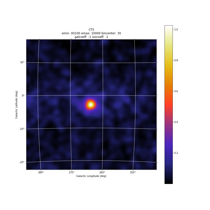
‘.cts.gz’ file
Counts maps are generated by the procedure AG_ctsmapgen embedded into Agilpy.
AG_ctsmapgen reads the event files listed in the event file index (see “AGILE data” section), bins the counts between tmin and tmax, and outputs a FITS image file. The image is a two-dimensional array in the ARC or AIT projection. The projection, size and resolution, the center and rotation of the map in Galactic coordinates, tmin, tmax, emin, and emax, along with various integration parameters (fovrad, fovradmin, albrad, phasecode) are managed by Agilepy.
The parameters are described in the “Configuration file” section.
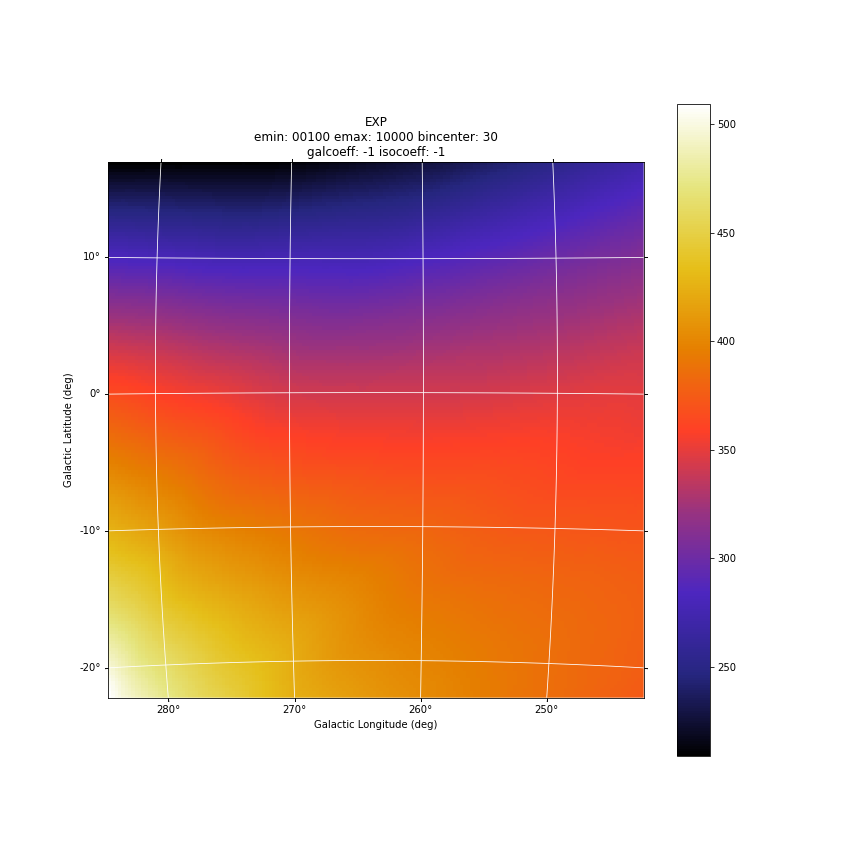
‘.exp.gz’ file
Exposure maps are generated by the procedure AG_expmapgen embedded into Agilpy.
The task AG_expmapgen reads the log files listed in the LOG index (see “AGILE data” section), integrates the exposure between tmin and tmax, and outputs a FITS exposure image file. The image is a two-dimensional array in either the ARC or AIT projection. The projection, size and resolution, and center and rotation of the map in Galactic coordinates, tmin, tmax, emin, emax, and index file are managed by Agilepy, along with various integration parameters (fovrad, albrad, y tol, roll tol, earth tol, phasecode), and an interpolation step size (binstep). The interpolation procedure is a linear interpolation method in which only one bin each N is calculated (where N is the step size parameter). For a bin size of 0.5 deg or 0.25 deg with a step size of N = 4 it is possible to get a good approximation of the exposure map.
The parameters are described in the “Configuration file” section.
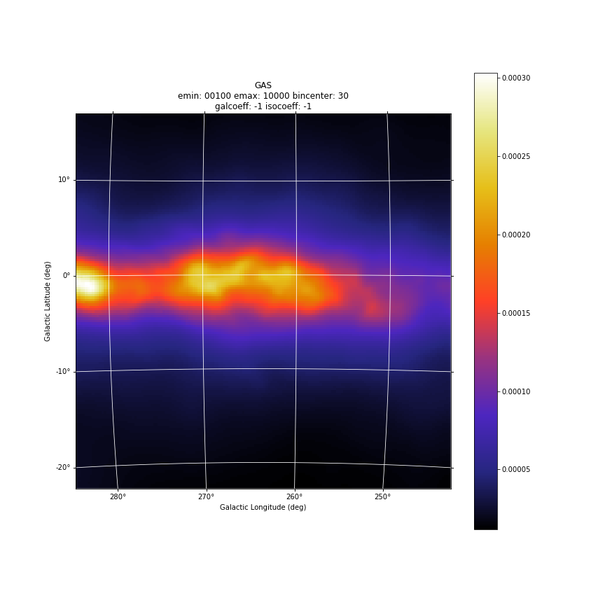
‘.gas.gz’ file
Diffuse emission maps are generated by the procedure AG_gasmapgen embedded into Agilpy. AG_gasmapgen reads an exposure map produced by AG_expmapgen and the master diffuse emission map and outputs a FITS image file, in the same format as the exposure map, in which each pixel contains the diffuse emission in that pixel. The image is a square array in the ARC projection. The diffuse emission map contain models of the diffuse emission convolved with the energy-dependent point spread function and combined into predefined observed energy ranges according to the appropriate energy dispersion function for G events using the FM3.119 background filter. The diffuse emission map automatically selected by Agilepy based on the energy range of the analysis; e.g. if the analysis is performed between 100 MeV and 50 GeV, Agilepy select the file 100_50000.0.1.SFMG_H0025.conv.sky.gz. The first number in the file name is the minimum energy and the second number is the maximum energy, followed by the resolution of the maps (0.1), the background event rejection filter (FM3.119) and the instrument response functions (IRFs).
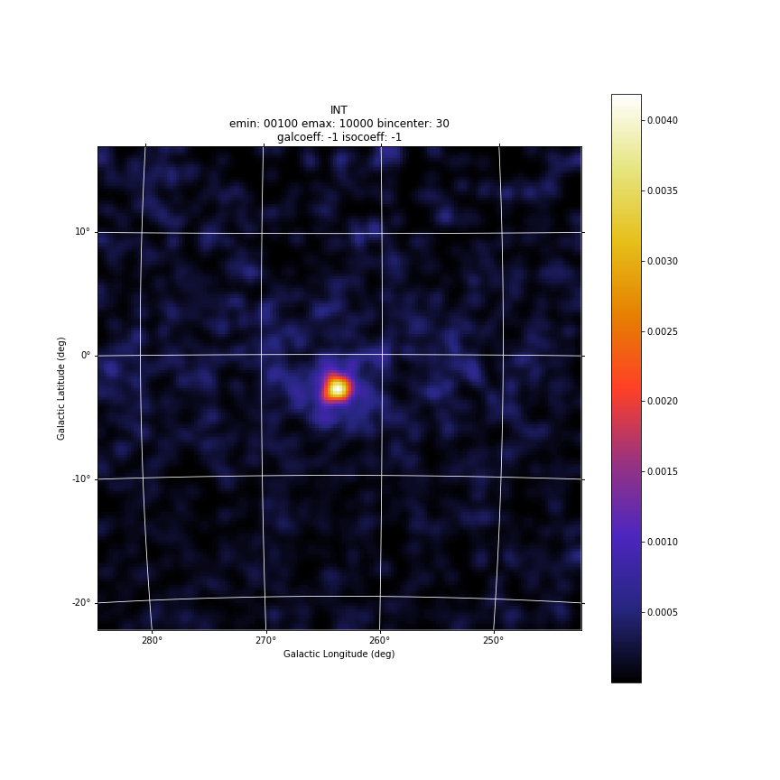
‘.int.gz’ file
Intensity maps are generated by the procedure AG_intmapgen embedded into Agilepy. AG_intmapgen reads an exposure map produced by AG_expmapgen and a counts map produced by AG_ctsmapgen and outputs a FITS image file, in the same format as the counts map, in which each pixel contains the intensity in that pixel. The image is a square array in the ARC projection. The two input maps should have been produced using the same set of parameters. The intensity map is not used in scientific analysis; it is useful solely as a visualization tool.
Light curves
AGILE-GRID light curves can be created in two different ways:
using a maximum likelihood estimator analysis
using aperture photometry.
The likelihood analysis reach better sensitivity, more accurate flux measurement, better evaluation of the backgrounds and can work with a detailed source models where more sources can be considered at the same time.
Aperture photometry provides a raw measure of the flux of a sigle source and is less computing demanding.
The likelihood light curve file contains the results of the generation of a light curve. The columns are the following:
time start (MJD)
time end (MJD)
sqrt(ts): the square root of the Test Statistic value of the results of the maximum likelihood estimator (mle)
flux (ph/cm2/s/sr)
flux_err (ph/cm2/s/sr)
flux_ul (ph/cm2/s/sr)
the value of the galactic diffuse emission (gal) parameter
the value of the isotropic emission (iso) parameter
position in Galactic coordinate (l_peak, b_peak): peak coordinates. If it is allowed to vary then they are set to the position for which the TS is maximized.
position in Galactic coordinate (l, b): evaluated by mle with the determination of the 95% confidence level elliptical confidence region
Radius (r) of 95% c.l. circular confidence region, deg. Statistical error only
ell_dist: the distance between (l,b) and the initial position
time start (UTC)
time end (UTC)
time start (TT)
time end (TT)
time_start_mjd time_end_mjd sqrt(ts) flux flux_err flux_ul gal iso l_peak b_peak dist l b r ell_dist time_start_utc time_end_utc time_start_tt time_end_tt
58026.49921296296 58027.49921296296 7.34802 944.077e-08 213.086e-08 1418.53e-08 0.7,0.7 4.08416,3.84041 263.647 -2.8547 0.0 -1.0 -1.0 -1.0 -1.0 2017-09-30T11:58:52 2017-10-01T11:58:52 433857532.0 433943932.0
58027.49921296296 58028.49921296296 8.88107 1054.87e-08 211.633e-08 1523.64e-08 0.7,0.7 4.08416,3.84041 263.647 -2.8547 0.0 -1.0 -1.0 -1.0 -1.0 2017-10-01T11:58:52 2017-10-02T11:58:52 433943932.0 434030332.0
58028.49921296296 58029.49921296296 7.31826 820.89e-08 198.193e-08 1266.73e-08 0.7,0.7 4.08416,3.84041 263.647 -2.8547 0.0 -1.0 -1.0 -1.0 -1.0 2017-10-02T11:58:52 2017-10-03T11:58:52 434030332.0 434116732.0
58029.49921296296 58030.49921296296 6.7938 840.137e-08 208.073e-08 1306.49e-08 0.7,0.7 4.08416,3.84041 263.647 -2.8547 0.0 -1.0 -1.0 -1.0 -1.0 2017-10-03T11:58:52 2017-10-04T11:58:52 434116732.0 434203132.0
58030.49921296296 58031.49921296296 7.62835 820.045e-08 190.836e-08 1249.26e-08 0.7,0.7 4.08416,3.84041 263.647 -2.8547 0.0 -1.0 -1.0 -1.0 -1.0 2017-10-04T11:58:52 2017-10-05T11:58:52 434203132.0 434289532.0
Result of the Maximum Likelihood Estimator
Agilepy shows a high-level view of the results of the maximum likelihood estimator. The details of the output of the science tool AG_multi that performs the likelihood procedure is still accessible. This section describes the “low level” results of the AG_multi procedure. The results are available in the $HOME/agilepy_analysis/<sourcename>_<username>_<date>-<time>/mle directory, where <sourcename> and <username> are defined in the yaml configuration file, <date> and <time> are defined by the system when the analysis starts.
At the end of the fitting process AG_multi generates two main files, describing the most relevant results for all the sources, and a set of source-specific files containing more detailed data about that source.
One of the two main files is in HTML format, and it includes both the input and output data grouped in tables. Having a look at this file the user should quickly understand the outcome of the fitting process and its main results. The next section describes the HTML output in more detail.
The second of the two main files contains the same data printed in text format. This file is divided in two sections. The first contains one line for each diffuse component and the second one line for each source. The first line of each section begins with an exclamation mark (a comment line for many applications) labeling the values printed beneath. In each line the values are separated by a space. This is an example of the text output of the analysis of the 2AGLJ2254+1609 (3C454.3) with the test dataset provided. For this analysis, only one set of maps and one source is used. The iotropic emission components coefficients are kep free and symmetric errors are provided. The flux and position of the source are allowed to vary, while the spectral index is fixed. The name, significance of the source detection, position, source counts with error, source flux with error, and spectral index with error are provided.
! DiffName, Flux, Err, +Err, -Err
Galactic 0.7 0 0 0
Isotropic 8.79898 0.969867 0.984804 -0.955381
! SrcName, sqrt(TS), L_peak, B_peak, Counts, Err, Flux, Err, Index, Err, Par2, Par2Err, Par3, Par3Err, TypeFun
2AGLJ2254+1609 35.5482 86.0638 -38.1753 719.369 35.2059 2.63371e-05 1.28894e-06 2.20942 0 0 0 0 0 0
index, par2, par3 and related errors depend by the spectral mode used.
The counts and fluxes are provided, as well as their errors if the flux is allowed to vary. Finally, the spectral index and its error, if applicable, are provided.
Note
If a source is outside the Galactic plane, fix the diffuse emission coefficient parameter (gal) to 0.7 with ag.setOptions(galcoeff=[0.7])
‘.source’ file
The .source file is an internal technical file produced by the maximum likelihood estimator mle() procedure for each source. It contains all the analysis results for each source that is part of the ensemble of models. Agilepy extract from this .source file the most important parameters useful for the final user.
When possible, two additional files describing the source contour (possibile only if position is kept free).
The text file contains some comment-like lines (first character is an exclamation mark) labeling the values printed beneath. This is an example of text output, consistent with the example given above:
! Label Fix index ULConfidenceLevel SrcLocConfLevel start_l start_b start_flux [ lmin,  lmax ] [ bmin, bmax ] typefun par2 par3 galmode2 galmode2fit isomode2 isomode2fit edpcor fluxcor integratortype expratioEval expratio_minthr expratio_maxthr expratio_size [ index_min , index_max ] [ par2_min , par2_max ] [ par3_min , par3_max ] contourpoints minimizertype minimizeralg minimizerdefstrategy minimizerdeftol
! sqrt(TS)
! L_peak B_peak Dist_from_start_position
! L B Dist_from_start_position r a b phi
! Counts Err +Err -Err UL
! Flux(ph/cm2s) [0 , 1e+07] Err +Err -Err UL(ph/cm2s) ULbayes(ph/cm2s) Exp(cm2s) ExpSpectraCorFactor null null null Erglog(erg/cm2s) Erglog_Err Erglog_UL(erg/cm2s) Sensitivity FluxPerChannel(ph/cm2s)
! Index [0.5 , 5] Index_Err Par2 [20 , 10000] Par2_Err Par3 [0 , 100] Par3_Err
! cts fitstatus0 fcn0 edm0 nvpar0 nparx0 iter0 fitstatus1 fcn1 edm1 nvpar1 nparx1 iter1 Likelihood1
! Gal coeffs [0 , 100] and errs
! Gal zero coeffs and errs
! Iso coeffs [0 , 100] and errs
! Iso zero coeffs and errs
! Start_date(UTC) End_date(UTC) Start_date(TT) End_date(TT) Start_date(MJD) End_date(MJD)
! Emin..emax(MeV) fovmin..fovmax(deg) albedo(deg) binsize(deg) expstep phasecode ExpRatio
! Fit status of steps ext1, step1, ext2, step2, contour, index, ul [-1 step skipped, 0 ok, 1 errors]
! Number of counts for each step (to evaluate hypothesis)
! skytypeL.filter_irf skytypeH.filter_irf
2AGLJ2254+1609 1 2.20942 2 5.99147 86.1236 -38.1824 2.64387e-05 [ -1 , -1 ]  [ -1 , -1 ]  0 0 0 0 0 0 0 0.75 0 1 1 0 15 10 [ 0.5 , 5 ] [ 20 , 10000 ] [ 0 , 100 ] 40 Minuit Migrad 2 0.01
47.8468
86.1236 -38.1824 0
-1 -1 -1 -1 -1 -1 -1
718.633 31.0247 31.4119 -30.6392 782.234
2.64387e-05 1.14141e-06 1.15565e-06 -1.12722e-06 2.87787e-05 2.01487e-05 2.71811e+07 1 0 0 0 4.27293e-09 1.8447e-10 4.6511e-09 0.0 2.64387e-05
2.20942 0 0 0 0 0
909 -1 2456.44 0.5 0 8 3 0 1311.78 7.28513e-16 1 8 3 1828.16
0.7 0
0.7 0
8.83231 0
8.83231 0
2010-11-13T00:01:06 2010-11-21T00:01:06 216691200.0000000 217382400.0000000 55513.0000000 55521.0000000
100..10000 0..60 80 0.25 0 6 0
-1 -1 -1 0 -1 -1 0
-1 2124 -1 2124 -1 -1 2124
SKY002.SFMG_H0025 SKY002.SFMG_H0025
The counts and fluxes are provided, as well as their symmetric, positive, and negative errors if the flux is allowed to vary. For convenience, the exposure of the source, used to calculate the source counts from the flux, is also provided. Finally, the spectral index and its error, if applicable, are provided.
Confidence Contour files
If a confidence contour was found, the parameters on the following line describe the best-fit ellipse of the contour, described in detail below.
If source location was requested for a given source and a source location contour was found, then three additional files are generated for that source. These files are written using galactic coordinates in degrees and can be loaded by applications such as ds9 and overlaid on the maps provided as input to AG_multi to visualize the source location contours. One of the three files, with extension .con, contains the source contour as found by the ROOT functions, expressed as a list of galactic coordinates, one point per line, where the last line is a repetition of the first. It may depict any shape. The other two files describe the ellipse that best fits the contour. One has extension .ellipse.con and represents the ellipse as a contour in a format analogous to that of the .con file. The other has extension .reg and describes same ellipse by its axes and orientation.
Determination of the ellipse. If AG_multi was able to find a source contour, an ellipse is fit to the contour. The source contour is a list of points which defines a polygon by connecting each point sequentially. The value of Radius found in the HTML output is the radius in degrees of a circle with the same area as the polygon. AG_multi determines the ellipse which best fits the contour. This ellipse will have the same area as the polygon, and the distance between each contour point and the intersection between the ellipse and the line connecting that point to the centre will be minimized. The ellipse is completely described by three parameters: the two axes and the rotation (in degrees) of the first axis around the centre, as expected by the ds9 application. If the ellipse is a circle, its axes will both be equal to the Radius found in the HTML output. The ellipse is described by two files that are readable by ds9: one is a .reg file which contains the centre, the axes and the rotation of the ellipse, while the other describes the same ellipse as a list of points in galactic coordinates, thus using the same syntax of a contour file, and has extension .ellipse.con. This is an example of ellipse .reg file:
HTML output. Additional details
The HTML output file is divided into two sections, input and output. The input section contains three subsections: the command line options, the map list and the source list contents. The command line options are listed in two tables, one with the names of the IRFs (PSD, SAR and EDP) files, the other with the rest of the command line. The maplist subsection also contains two tables. The first lists the mapfile contents and the second contains the data from the map files themselves. This table contains one map per row, and each column contains one value only if it is the same for all the maps. The last table of the input section contains the source list contents. The output section is also divided into three subsections. The first is a table showing the Galactic and isotropic coefficients and their errors. Also in this table some cells may be grouped together when the values are all the same. The second is a table showing the fit results for the sources and their errors. One of the listed values is the contour equivalent radius, explained in the next section. The last table shows the source flux per energy channel, and it is present only when different energy channels are considered. This table has one row for each source and one column for each energy channel.
Data files
‘.maplist4’ file
The map list is a text file listing containing at least one line of text. Each line of text describes one set of maps and it is possible to include empty lines or comment lines. The comment lines begin with an exclamation mark.
Each line contains a set of maps:
<countsMap> <exposureMap> <gasMap> <offaxisangle> <galcoeff> <isocoeff>
where:
countsMap, exposureMap and gasMap are file system paths pointing to the corresponding sky maps (see SkyMaps section)
offaxisangle is in degrees;
galcoeff and isocoeff are the coefficients for the galactic and isotropic diffuse components. If positive they will be considered fixed (but see galmode and isomode section).